What Happens To The Critical Value For A Chi-square Test If The Size Of The Sample Is Increased?

Hypothesis Testing - Chi Squared Test

Author:

Lisa Sullivan, PhD

Professor of Biostatistics

Boston University Schoolhouse of Public Health

Introduction

---

This module will continue the discussion of hypothesis testing, where a specific statement or hypothesis is generated about a population parameter, and sample statistics are used to appraise the likelihood that the hypothesis is true. The hypothesis is based on available information and the investigator's belief about the population parameters. The specific tests considered here are chosen chi-square tests and are appropriate when the outcome is discrete (dichotomous, ordinal or categorical). For example, in some clinical trials the outcome is a nomenclature such as hypertensive, pre-hypertensive or normotensive. We could apply the same classification in an observational study such equally the Framingham Middle Study to compare men and women in terms of their blood pressure level status - once again using the classification of hypertensive, pre-hypertensive or normotensive status.

The technique to analyze a detached event uses what is called a chi-square test. Specifically, the test statistic follows a chi-square probability distribution. We will consider chi-foursquare tests hither with ane, ii and more than than two contained comparison groups.

Learning Objectives

---

After completing this module, the pupil volition exist able to:

1. Perform chi-square tests by manus
2. Appropriately interpret results of chi-square tests
3. Identify the appropriate hypothesis testing procedure based on type of event variable and number of samples

Tests with Ane Sample, Discrete Outcome

---

Here we consider hypothesis testing with a discrete outcome variable in a single population. Detached variables are variables that take on more than two distinct responses or categories and the responses can be ordered or unordered (i.due east., the outcome can exist ordinal or chiselled). The process nosotros describe here can be used for dichotomous (exactly ii response options), ordinal or chiselled discrete outcomes and the objective is to compare the distribution of responses, or the proportions of participants in each response category, to a known distribution. The known distribution is derived from another report or study and it is again important in setting up the hypotheses that the comparator distribution specified in the cipher hypothesis is a off-white comparison. The comparator is sometimes chosen an external or a historical command.

In one sample tests for a detached consequence, nosotros prepare up our hypotheses against an advisable comparator. We select a sample and compute descriptive statistics on the sample data. Specifically, we compute the sample size (n) and the proportions of participants in each response

category ( , , ... ) where 1000 represents the number of response categories. We then determine the advisable examination statistic for the hypothesis test. The formula for the test statistic is given below.

Exam Statistic for Testing H₀: p₁ = p ₁₀ , p₂ = p _xx , ..., p_k = p _k0

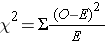
We find the critical value in a table of probabilities for the chi-square distribution with degrees of freedom (df) = g-1. In the exam statistic, O = observed frequency and East=expected frequency in each of the response categories. The observed frequencies are those observed in the sample and the expected frequencies are computed as described below. χ² (chi-square) is some other probability distribution and ranges from 0 to ∞. The examination higher up statistic formula to a higher place is appropriate for big samples, divers equally expected frequencies of at least 5 in each of the response categories.

When we conduct a χ² test, we compare the observed frequencies in each response category to the frequencies we would expect if the null hypothesis were truthful. These expected frequencies are determined by allocating the sample to the response categories according to the distribution specified in H₀. This is washed by multiplying the observed sample size (n) by the proportions specified in the zip hypothesis (p ₁₀ , p ₂₀ , ..., p _k0 ). To ensure that the sample size is appropriate for the use of the exam statistic above, we need to ensure that the following: min(np_ten , n p₂₀ , ..., north p_k0 ) > 5.

The examination of hypothesis with a discrete consequence measured in a single sample, where the goal is to assess whether the distribution of responses follows a known distribution, is called the χ² goodness-of-fit examination. Every bit the proper name indicates, the idea is to assess whether the pattern or distribution of responses in the sample "fits" a specified population (external or historical) distribution. In the next example we illustrate the test. As we work through the instance, nosotros provide additional details related to the apply of this new test statistic.

Example:

A Academy conducted a survey of its recent graduates to collect demographic and health data for future planning purposes as well as to assess students' satisfaction with their undergraduate experiences. The survey revealed that a substantial proportion of students were not engaging in regular exercise, many felt their nutrition was poor and a substantial number were smoking. In response to a question on regular exercise, 60% of all graduates reported getting no regular practice, 25% reported exercising sporadically and 15% reported exercising regularly as undergraduates. The side by side twelvemonth the University launched a health promotion campaign on campus in an attempt to increment wellness behaviors amidst undergraduates. The plan included modules on practice, nutrition and smoking cessation. To evaluate the impact of the program, the University again surveyed graduates and asked the same questions. The survey was completed by 470 graduates and the following data were collected on the practice question:

	No Regular Practise	Desultory Exercise	Regular Exercise	Total
Number of Students	255	125	ninety	470

Based on the information, is there evidence of a shift in the distribution of responses to the practice question following the implementation of the wellness promotion entrada on campus? Run the examination at a 5% level of significance.

In this example, we have one sample and a detached (ordinal) result variable (with three response options). We specifically desire to compare the distribution of responses in the sample to the distribution reported the previous year (i.e., sixty%, 25%, 15% reporting no, sporadic and regular practise, respectively). Nosotros now run the test using the five-footstep approach.

• Stride 1. Set up hypotheses and determine level of significance.

The nothing hypothesis again represents the "no change" or "no difference" situation. If the health promotion entrada has no bear on and so nosotros look the distribution of responses to the exercise question to be the same as that measured prior to the implementation of the program.

H₀: p₁=0.threescore, p₂=0.25, p_iii=0.xv,  or equivalently H₀: Distribution of responses is 0.60, 0.25, 0.15

H₁:   H₀ is faux.          α =0.05

Notice that the inquiry hypothesis is written in words rather than in symbols. The inquiry hypothesis equally stated captures any divergence in the distribution of responses from that specified in the null hypothesis. Nosotros do not specify a specific alternative distribution, instead we are testing whether the sample information "fit" the distribution in H₀ or not. With the χⁱⁱ goodness-of-fit test there is no upper or lower tailed version of the exam.

• Step 2. Select the advisable test statistic.

The test statistic is:

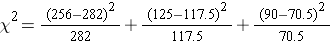
We must first assess whether the sample size is adequate. Specifically, we need to bank check min(np₀, np_i, ..., n p₁₀₀₀) > 5. The sample size here is north=470 and the proportions specified in the null hypothesis are 0.60, 0.25 and 0.fifteen. Thus, min( 470(0.65), 470(0.25), 470(0.xv))=min(282, 117.v, 70.v)=70.five. The sample size is more than adequate and then the formula can be used.

• Step 3. Set up up decision rule.

The decision rule for the χⁱⁱ test depends on the level of significance and the degrees of freedom, defined equally degrees of freedom (df) = one thousand-1 (where k is the number of response categories). If the null hypothesis is true, the observed and expected frequencies volition be shut in value and the χ² statistic volition be close to null. If the null hypothesis is imitation, then the χ² statistic will be large. Critical values can be found in a table of probabilities for the χ^two distribution. Here nosotros have df=1000-1=iii-1=2 and a 5% level of significance. The appropriate critical value is 5.99, and the decision rule is as follows: Pass up H₀ if χ^two > 5.99.

• Step 4. Compute the exam statistic.

Nosotros now compute the expected frequencies using the sample size and the proportions specified in the null hypothesis. We and so substitute the sample data (observed frequencies) and the expected frequencies into the formula for the test statistic identified in Stride 2. The computations can be organized as follows.

	No Regular Exercise	Sporadic Practice	Regular Practise	Total
Observed Frequencies (O)	255	125	90	470
Expected Frequencies (E)	470(0.threescore) =282	470(0.25) =117.5	470(0.15) =70.5	470

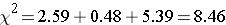
Detect that the expected frequencies are taken to one decimal place and that the sum of the observed frequencies is equal to the sum of the expected frequencies. The exam statistic is computed as follows:

• Step 5. Conclusion.

We reject H₀ because 8.46 > 5.99. Nosotros have statistically significant evidence at α=0.05 to bear witness that H₀ is false, or that the distribution of responses is not 0.lx, 0.25, 0.15.  The p-value is p < 0.005.

In the χ² goodness-of-fit test, we conclude that either the distribution specified in H₀ is simulated (when we decline H₀) or that we do non have sufficient evidence to show that the distribution specified in H₀ is false (when nosotros fail to decline H₀). Here, we refuse H₀ and ended that the distribution of responses to the do question following the implementation of the wellness promotion entrada was non the aforementioned every bit the distribution prior. The exam itself does not provide details of how the distribution has shifted. A comparison of the observed and expected frequencies will provide some insight into the shift (when the null hypothesis is rejected). Does information technology announced that the wellness promotion campaign was constructive?

Consider the following:

	No Regular Do	Sporadic Practice	Regular Exercise	Total
Observed Frequencies (O)	255	125	90	470
Expected Frequencies (Eastward)	282	117.5	70.5	470

If the null hypothesis were true (i.e., no alter from the prior year) we would have expected more students to fall in the "No Regular Practise" category and fewer in the "Regular Exercise" categories. In the sample, 255/470 = 54% reported no regular exercise and 90/470=nineteen% reported regular practise. Thus, in that location is a shift toward more regular exercise post-obit the implementation of the health promotion entrada. There is bear witness of a statistical difference, is this a meaningful difference? Is there room for improvement?

Example:

The National Center for Health Statistics (NCHS) provided data on the distribution of weight (in categories) among Americans in 2002. The distribution was based on specific values of body mass alphabetize (BMI) computed as weight in kilograms over pinnacle in meters squared. Underweight was defined as BMI< 18.v, Normal weight equally BMI between 18.5 and 24.nine, overweight as BMI betwixt 25 and 29.9 and obese equally BMI of 30 or greater. Americans in 2002 were distributed every bit follows: 2% Underweight, 39% Normal Weight, 36% Overweight, and 23% Obese. Suppose we desire to assess whether the distribution of BMI is unlike in the Framingham Offspring sample. Using information from the northward=3,326 participants who attended the seventh examination of the Offspring in the Framingham Eye Study nosotros created the BMI categories as defined and observed the post-obit:

	Underweight BMI<18.5	Normal Weight BMI 18.5-24.nine	Overweight BMI 25.0-29.9	Obese BMI > 30	Total
# of Participants	20	932	1374	one thousand	3326

• Step one. Fix hypotheses and decide level of significance.

H₀: p_ane=0.02, p_ii=0.39, p₃=0.36, p₄=0.23     or equivalently

H₀: Distribution of responses is 0.02, 0.39, 0.36, 0.23

H₁:   H₀ is false.        α=0.05

• Footstep ii. Select the advisable exam statistic.

The formula for the test statistic is:

We must assess whether the sample size is acceptable. Specifically, nosotros need to check min(np₀, np_1, ..., north p_thousand) > v. The sample size here is north=three,326 and the proportions specified in the nix hypothesis are 0.02, 0.39, 0.36 and 0.23. Thus, min( 3326(0.02), 3326(0.39), 3326(0.36), 3326(0.23))=min(66.5, 1297.1, 1197.4, 765.0)=66.5. The sample size is more than adequate, then the formula can be used.

• Step 3. Prepare upwardly conclusion rule.

Here we have df=thou-1=4-1=3 and a 5% level of significance. The appropriate critical value is 7.81 and the decision rule is equally follows: Reject H₀ if χⁱⁱ > seven.81.

• Footstep 4. Compute the test statistic.

Nosotros now compute the expected frequencies using the sample size and the proportions specified in the zilch hypothesis. We so substitute the sample data (observed frequencies) into the formula for the examination statistic identified in Footstep 2. We organize the computations in the following table.

	Underweight BMI<18.5	Normal BMI xviii.five-24.9	Overweight BMI 25.0-29.ix	Obese BMI > thirty	Full
Observed Frequencies (O)	20	932	1374	1000	3326
Expected Frequencies (Eastward)	66.5	1297.1	1197.four	765.0	3326

The test statistic is computed every bit follows:

• Footstep v. Decision.

We decline H₀ because 233.53 > 7.81. Nosotros accept statistically pregnant evidence at α=0.05 to evidence that H₀ is false or that the distribution of BMI in Framingham is dissimilar from the national data reported in 2002, p < 0.005.

Once more, the χⁱⁱgoodness-of-fit examination allows united states to assess whether the distribution of responses "fits" a specified distribution. Hither we evidence that the distribution of BMI in the Framingham Offspring Study is different from the national distribution. To understand the nature of the divergence we tin compare observed and expected frequencies or observed and expected proportions (or percentages). The frequencies are large considering of the large sample size, the observed percentages of patients in the Framingham sample are every bit follows: 0.6% underweight, 28% normal weight, 41% overweight and 30% obese. In the Framingham Offspring sample in that location are college percentages of overweight and obese persons (41% and 30% in Framingham as compared to 36% and 23% in the national information), and lower proportions of underweight and normal weight persons (0.six% and 28% in Framingham as compared to 2% and 39% in the national data). Are these meaningful differences?

In the module on hypothesis testing for ways and proportions, we discussed hypothesis testing applications with a dichotomous outcome variable in a single population. Nosotros presented a test using a test statistic Z to test whether an observed (sample) proportion differed significantly from a historical or external comparator. The chi-foursquare goodness-of-fit test tin also be used with a dichotomous outcome and the results are mathematically equivalent.

In the prior module, nosotros considered the following example. Here we prove the equivalence to the chi-foursquare goodness-of-fit test.

Example:

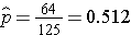
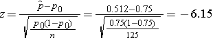
The NCHS report indicated that in 2002, 75% of children aged 2 to 17 saw a dentist in the past year. An investigator wants to assess whether use of dental services is similar in children living in the city of Boston. A sample of 125 children aged 2 to 17 living in Boston are surveyed and 64 reported seeing a dentist over the by 12 months. Is there a meaning difference in use of dental services betwixt children living in Boston and the national information?

We presented the following approach to the test using a Z statistic.

• Step i. Fix hypotheses and determine level of significance

H₀: p = 0.75

H₁: p ≠ 0.75                               α=0.05

• Stride 2. Select the advisable examination statistic.

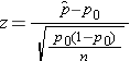
We must kickoff check that the sample size is adequate. Specifically, we need to check min(np₀, due north(1-p₀)) = min( 125(0.75), 125(1-0.75))=min(94, 31)=31. The sample size is more than adequate so the post-obit formula tin can be used

• Step 3. Set up decision rule.

This is a two-tailed test, using a Z statistic and a five% level of significance. Decline H₀ if Z < -one.960 or if Z > 1.960.

• Footstep 4. Compute the exam statistic.

We at present substitute the sample data into the formula for the test statistic identified in Step 2. The sample proportion is:

• Footstep 5. Conclusion.

We reject H₀ considering -6.15 < -i.960. We have statistically significant testify at a =0.05 to evidence that there is a statistically meaning difference in the use of dental service by children living in Boston as compared to the national information. (p < 0.0001).

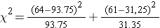
We at present conduct the same test using the chi-square goodness-of-fit test. First, we summarize our sample information as follows:

	Saw a Dentist in Past 12 Months	Did Not Run across a Dentist in By 12 Months	Total
# of Participants	64	61	125

• Footstep 1. Ready hypotheses and determine level of significance.

H₀: p₁=0.75, p_ii=0.25     or equivalently H₀: Distribution of responses is 0.75, 0.25

H₁:   H₀ is false.        α=0.05

• Step ii. Select the appropriate exam statistic.

The formula for the test statistic is:

We must assess whether the sample size is adequate. Specifically, nosotros need to bank check min(np₀, np_ane, ...,np_k>) > 5. The sample size here is n=125 and the proportions specified in the zero hypothesis are 0.75, 0.25. Thus, min( 125(0.75), 125(0.25))=min(93.75, 31.25)=31.25. The sample size is more than adequate so the formula can be used.

• Step 3. Ready decision dominion.

Hither we have df=k-1=2-i=i and a 5% level of significance. The appropriate disquisitional value is 3.84, and the determination rule is as follows: Turn down H₀ if χⁱⁱ > 3.84. (Note that 1.96² = iii.84, where 1.96 was the disquisitional value used in the Z exam for proportions shown in a higher place.)

• Step 4. Compute the examination statistic.

We at present compute the expected frequencies using the sample size and the proportions specified in the zilch hypothesis. We and then substitute the sample information (observed frequencies) into the formula for the test statistic identified in Step 2. Nosotros organize the computations in the following table.

	Saw a Dentist in Past 12 Months	Did Not Run across a Dentist in Past 12 Months	Total
Observed Frequencies (O)	64	61	125
Expected Frequencies (E)	93.75	31.25	125

The exam statistic is computed as follows:

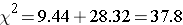
(Notation that (-6.15)² = 37.8, where -6.15 was the value of the Z statistic in the examination for proportions shown above.)

• Stride v. Conclusion.

Nosotros reject H₀ considering 37.8 > 3.84. We have statistically meaning evidence at α=0.05 to prove that there is a statistically significant difference in the use of dental service by children living in Boston as compared to the national data.  (p < 0.0001). This is the aforementioned conclusion we reached when we conducted the examination using the Z examination above. With a dichotomous outcome, Z² = χ² !   In statistics, there are often several approaches that tin can exist used to test hypotheses.

Tests for Two or More Contained Samples, Discrete Consequence

---

Here nosotros extend that application of the chi-foursquare exam to the example with two or more independent comparison groups. Specifically, the outcome of interest is detached with two or more responses and the responses can be ordered or unordered (i.eastward., the outcome can be dichotomous, ordinal or categorical). We now consider the situation where there are two or more than contained comparison groups and the goal of the analysis is to compare the distribution of responses to the discrete result variable among several independent comparison groups.

The test is called the χⁱⁱ examination of independence and the nix hypothesis is that there is no difference in the distribution of responses to the outcome beyond comparison groups. This is often stated equally follows: The consequence variable and the group variable (due east.grand., the comparing treatments or comparison groups) are independent (hence the name of the test). Independence here implies homogeneity in the distribution of the outcome among comparison groups.

The nil hypothesis in the χ² exam of independence is frequently stated in words as: H₀: The distribution of the outcome is independent of the groups. The alternative or inquiry hypothesis is that there is a difference in the distribution of responses to the outcome variable among the comparison groups (i.eastward., that the distribution of responses "depends" on the group). In order to examination the hypothesis, we measure the discrete outcome variable in each participant in each comparison group. The information of interest are the observed frequencies (or number of participants in each response category in each grouping). The formula for the test statistic for the χ^two test of independence is given below.

Test Statistic for Testing H₀: Distribution of outcome is independent of groups

and we find the critical value in a table of probabilities for the chi-square distribution with df=(r-ane)*(c-1).

Here O = observed frequency, E=expected frequency in each of the response categories in each group, r = the number of rows in the two-manner tabular array and c = the number of columns in the two-way table.   r and c correspond to the number of comparing groups and the number of response options in the outcome (see below for more than details). The observed frequencies are the sample data and the expected frequencies are computed equally described below. The test statistic is appropriate for large samples, divers as expected frequencies of at least 5 in each of the response categories in each group.

The data for the χ² test of independence are organized in a 2-style tabular array. The upshot and group variable are shown in the rows and columns of the tabular array. The sample table below illustrates the data layout. The table entries (blank below) are the numbers of participants in each grouping responding to each response category of the outcome variable.

Table - Possible outcomes are are listed in the columns; The groups beingness compared are listed in rows.

	Outcome Variable
Grouping Variable	Response Option 1	Response Option 2	...	Response Option c	Row Totals
Group one
Grouping 2
. . .
Group r
Column Totals					N

In the table above, the grouping variable is shown in the rows of the tabular array; r denotes the number of independent groups. The outcome variable is shown in the columns of the table; c denotes the number of response options in the outcome variable. Each combination of a row (grouping) and cavalcade (response) is called a jail cell of the table. The table has r*c cells and is sometimes chosen an r 10 c ("r by c") table. For example, if there are iv groups and five categories in the outcome variable, the data are organized in a 4 X 5 tabular array. The row and column totals are shown forth the right-manus margin and the bottom of the table, respectively. The total sample size, N, can be computed by summing the row totals or the column totals. Similar to ANOVA, N does not refer to a population size here just rather to the full sample size in the assay. The sample data can be organized into a table like the above. The numbers of participants inside each grouping who select each response selection are shown in the cells of the table and these are the observed frequencies used in the test statistic.

The test statistic for the χ² test of independence involves comparing observed (sample data) and expected frequencies in each cell of the table. The expected frequencies are computed assuming that the null hypothesis is truthful. The null hypothesis states that the two variables (the grouping variable and the outcome) are independent. The definition of independence is every bit follows:

 Two events, A and B, are independent if P(A|B) = P(A), or equivalently, if P(A and B) = P(A) P(B).

The second statement indicates that if two events, A and B, are independent then the probability of their intersection can be computed past multiplying the probability of each private effect. To conduct the χⁱⁱ test of independence, nosotros need to compute expected frequencies in each prison cell of the table. Expected frequencies are computed by bold that the grouping variable and issue are independent (i.eastward., under the zero hypothesis). Thus, if the goose egg hypothesis is truthful, using the definition of independence:

P(Grouping 1 and Response Option 1) = P(Group 1) P(Response Option 1).

 The above states that the probability that an individual is in Group 1 and their upshot is Response Option i is computed past multiplying the probability that person is in Group i by the probability that a person is in Response Option 1. To conduct the χ² test of independence, nosotros need expected frequencies and not expected probabilities. To catechumen the above probability to a frequency, we multiply by N. Consider the following small example.

	Response i	Response 2	Response iii	Total
Group 1	10	8	vii	25
Group 2	22	15	13	50
Group 3	30	28	17	75
Total	62	51	37	150

The data shown above are measured in a sample of size N=150. The frequencies in the cells of the tabular array are the observed frequencies. If Grouping and Response are contained, then we tin can compute the probability that a person in the sample is in Group 1 and Response category 1 using:

P(Group 1 and Response 1) = P(Group one) P(Response i),

P(Group i and Response 1) = (25/150) (62/150) = 0.069.

Thus if Grouping and Response are independent we would wait 6.9% of the sample to be in the top left prison cell of the table (Group 1 and Response one). The expected frequency is 150(0.069) = 10.iv.   We could do the same for Group 2 and Response 1:

P(Group 2 and Response 1) = P(Grouping 2) P(Response 1),

P(Group ii and Response 1) = (l/150) (62/150) = 0.138.

The expected frequency in Group ii and Response one is 150(0.138) = twenty.7.

Thus, the formula for determining the expected cell frequencies in the χⁱⁱ test of independence is as follows:

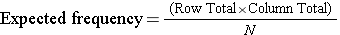
Expected Cell Frequency = (Row Total * Column Total)/Due north.

The above computes the expected frequency in one step rather than calculating the expected probability kickoff and and then converting to a frequency.

Case:

In a prior example we evaluated data from a survey of academy graduates which assessed, among other things, how frequently they exercised. The survey was completed past 470 graduates. In the prior example we used the χ² goodness-of-fit examination to assess whether there was a shift in the distribution of responses to the exercise question post-obit the implementation of a wellness promotion campaign on campus. We specifically considered one sample (all students) and compared the observed distribution to the distribution of responses the prior year (a historical control). Suppose we at present wish to assess whether there is a human relationship between exercise on campus and students' living arrangements. As office of the same survey, graduates were asked where they lived their senior year. The response options were dormitory, on-campus apartment, off-campus apartment, and at dwelling (i.e., commuted to and from the university). The data are shown beneath.

	No Regular Do	Sporadic Do	Regular Exercise	Total
Dormitory	32	30	28	90
On-Campus Flat	74	64	42	180
Off-Campus Flat	110	25	15	150
At Home	39	vi	5	50
Total	255	125	90	470

Based on the data, is there a relationship between exercise and student'south living arrangement? Do you think where a person lives affect their exercise status? Hither we have 4 contained comparison groups (living organisation) and a detached (ordinal) outcome variable with three response options. We specifically want to test whether living arrangement and exercise are independent. We will run the test using the v-step approach.

• Footstep i. Gear up hypotheses and make up one's mind level of significance.

H₀: Living system and exercise are independent

H_ane: H₀ is false.                α=0.05

The cypher and research hypotheses are written in words rather than in symbols. The enquiry hypothesis is that the grouping variable (living arrangement) and the outcome variable (do) are dependent or related.

• Step two. Select the appropriate test statistic.

The formula for the examination statistic is:

.

The condition for appropriate apply of the in a higher place exam statistic is that each expected frequency is at least 5. In Stride 4 we will compute the expected frequencies and we will ensure that the condition is met.

• Step 3. Set conclusion dominion.

The conclusion dominion depends on the level of significance and the degrees of freedom, defined equally df = (r-1)(c-one), where r and c are the numbers of rows and columns in the two-way data table.   The row variable is the living arrangement and there are 4 arrangements considered, thus r=4. The column variable is practice and iii responses are considered, thus c=three. For this exam, df=(four-1)(3-1)=3(2)=6. Over again, with χ² tests in that location are no upper, lower or two-tailed tests. If the null hypothesis is true, the observed and expected frequencies will be shut in value and the χ² statistic will be close to null. If the aught hypothesis is false, then the χ² statistic volition be large. The rejection region for the χ^two examination of independence is always in the upper (right-hand) tail of the distribution. For df=half-dozen and a five% level of significance, the advisable critical value is 12.59 and the decision rule is as follows: Reject H₀ if c ² > 12.59.

• Step 4. Compute the test statistic.

Nosotros now compute the expected frequencies using the formula,

Expected Frequency = (Row Full * Column Total)/N.

The computations can be organized in a two-style table. The top number in each jail cell of the table is the observed frequency and the bottom number is the expected frequency.   The expected frequencies are shown in parentheses.

	No Regular Exercise	Desultory Exercise	Regular Exercise	Full
Dormitory	32 (48.8)	xxx (23.9)	28 (17.2)	90
On-Campus Apartment	74 (97.7)	64 (47.nine)	42 (34.5)	180
Off-Campus Flat	110 (81.4)	25 (39.9)	15 (28.7)	150
At Home	39 (27.1)	6 (13.3)	5 (9.half dozen)	50
Total	255	125	90	470

Observe that the expected frequencies are taken to one decimal place and that the sums of the observed frequencies are equal to the sums of the expected frequencies in each row and column of the table.

Remember in Step two a condition for the appropriate use of the test statistic was that each expected frequency is at to the lowest degree 5. This is true for this sample (the smallest expected frequency is 9.6) and therefore it is appropriate to use the test statistic.

The test statistic is computed as follows:

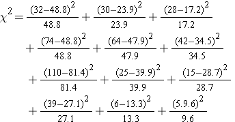
• Step 5. Conclusion.

We pass up H₀ because 60.v > 12.59. We accept statistically significant evidence at a =0.05 to testify that H₀ is simulated or that living arrangement and exercise are not independent (i.e., they are dependent or related), p < 0.005.

Again, the χ² test of independence is used to exam whether the distribution of the outcome variable is like across the comparison groups. Here we rejected H₀ and concluded that the distribution of do is not independent of living system, or that there is a relationship betwixt living system and exercise. The exam provides an overall assessment of statistical significance. When the aught hypothesis is rejected, it is important to review the sample information to sympathize the nature of the relationship. Consider once again the sample information.

	No Regular Practise	Sporadic Exercise	Regular Practise	Total
Dormitory	32	30	28	xc
On-Campus Apartment	74	64	42	180
Off-Campus Flat	110	25	15	150
At Habitation	39	6	5	50
Full	255	125	90	470

Because there are different numbers of students in each living state of affairs, it makes the comparisons of exercise patterns difficult on the basis of the frequencies lonely. The following table displays the percentages of students in each exercise category by living organization. The percentages sum to 100% in each row of the table. For comparing purposes, percentages are also shown for the total sample along the bottom row of the table.

	No Regular Exercise	Desultory Do	Regular Exercise
Dormitory	36%	33%	31%
On-Campus Apartment	41%	36%	23%
Off-Campus Apartment	73%	17%	10%
At Habitation	78%	12%	10%
Total	54%	27%	19%

From the in a higher place, it is clear that higher percentages of students living in dormitories and in on-campus apartments reported regular practice (31% and 23%) equally compared to students living in off-campus apartments and at dwelling (x% each).

Test Yourself

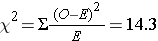
 Pancreaticoduodenectomy (PD) is a procedure that is associated with considerable morbidity. A written report was recently conducted on 553 patients who had a successful PD betwixt January 2000 and Dec 2010 to decide whether their Surgical Apgar Score (SAS) is related to 30-24-hour interval perioperative morbidity and bloodshed. The tabular array below gives the number of patients experiencing no, minor, or major morbidity by SAS category.

Surgical Apgar Score	No morbidity	Minor morbidity	Major morbidity or mortality
0-4	21	20	16
5-6	135	71	35
7-10	158	62	35

Question: What would be an appropriate statistical exam to examine whether there is an association between Surgical Apgar Score and patient outcome? Using 14.thirteen as the value of the examination statistic for these data, carry out the appropriate examination at a 5% level of significance. Show all parts of your test.

Answer

In the module on hypothesis testing for ways and proportions, we discussed hypothesis testing applications with a dichotomous outcome variable and two contained comparison groups. We presented a test using a test statistic Z to test for equality of contained proportions. The chi-square test of independence tin also exist used with a dichotomous outcome and the results are mathematically equivalent.

In the prior module, we considered the following example. Here we evidence the equivalence to the chi-square test of independence.

Case:

A randomized trial is designed to evaluate the effectiveness of a newly adult pain reliever designed to reduce pain in patients following joint replacement surgery. The trial compares the new pain reliever to the pain reliever currently in use (called the standard of care). A full of 100 patients undergoing joint replacement surgery agreed to participate in the trial. Patients were randomly assigned to receive either the new pain reliever or the standard pain reliever following surgery and were blind to the treatment consignment. Before receiving the assigned treatment, patients were asked to rate their pain on a calibration of 0-ten with higher scores indicative of more hurting. Each patient was so given the assigned treatment and afterward thirty minutes was again asked to rate their pain on the same scale. The primary effect was a reduction in pain of 3 or more scale points (defined by clinicians equally a clinically meaningful reduction). The following information were observed in the trial.

Handling Grouping	due north	Number with Reduction of iii+ Points	Proportion with Reduction of 3+ Points
New Hurting Reliever	50	23	0.46
Standard Pain Reliever	l	11	0.22

Nosotros tested whether there was a significant departure in the proportions of patients reporting a meaningful reduction (i.due east., a reduction of 3 or more than calibration points) using a Z statistic, as follows.

• Step 1. Prepare up hypotheses and determine level of significance

H₀: p₁ = p_ii

H_i: p₁ ≠ p₂ α=0.05

Here the new or experimental pain reliever is group 1 and the standard pain reliever is grouping ii.

• Step 2. Select the appropriate test statistic.

We must outset cheque that the sample size is acceptable. Specifically, we demand to ensure that we have at to the lowest degree five successes and 5 failures in each comparing grouping or that:

In this example, nosotros have

Therefore, the sample size is adequate, so the post-obit formula can exist used:

.

• Step 3. Set upward determination rule.

Refuse H₀ if Z < -1.960 or if Z > i.960.

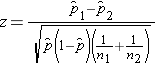
• Step 4. Compute the exam statistic.

We now substitute the sample information into the formula for the test statistic identified in Step ii. We beginning compute the overall proportion of successes:

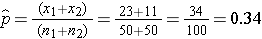
We now substitute to compute the exam statistic.

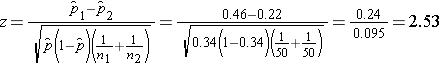
• Step 5. Conclusion.

Nosotros reject H₀ because . We take statistically significant testify at α=0.05 to show that in that location is a difference in the proportions of patients on the new hurting reliever reporting a meaningful reduction (i.e., a reduction of 3 or more scale points) every bit compared to patients on the standard pain reliever.

We at present acquit the same test using the chi-foursquare test of independence.

• Step ane. Set up hypotheses and determine level of significance.

H₀: Treatment and outcome (meaningful reduction in pain) are independent

H₁:   H₀ is false.         α=0.05

• Step 2. Select the appropriate exam statistic.

The formula for the examination statistic is:

The condition for appropriate apply of the above test statistic is that each expected frequency is at to the lowest degree 5. In Step four we volition compute the expected frequencies and nosotros will ensure that the condition is met.

• Stride iii. Gear up determination rule.

For this examination, df=(2-one)(2-1)=i. At a v% level of significance, the appropriate critical value is three.84 and the decision rule is as follows: Reject H0 if χ² > 3.84. (Note that i.96² = 3.84, where 1.96 was the critical value used in the Z examination for proportions shown higher up.)

• Step four. Compute the test statistic.

We at present compute the expected frequencies using:

The computations can be organized in a two-mode table. The top number in each cell of the tabular array is the observed frequency and the bottom number is the expected frequency. The expected frequencies are shown in parentheses.

Treatment Group	# with Reduction of three+ Points	# with Reduction of <3 Points	Total
New Hurting Reliever	23 (17.0)	27 (33.0)	50
Standard Hurting Reliever	11 (17.0)	39 (33.0)	l
Total	34	66	100

A status for the appropriate use of the test statistic was that each expected frequency is at to the lowest degree 5. This is true for this sample (the smallest expected frequency is 22.0) and therefore it is appropriate to use the test statistic.

The test statistic is computed equally follows:

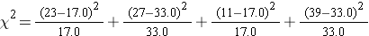
(Note that (ii.53)² = 6.4, where two.53 was the value of the Z statistic in the test for proportions shown to a higher place.)

• Footstep 5. Decision.

We turn down H₀ because . We take statistically pregnant evidence at α=0.05 to show that H₀ is simulated or that handling and outcome are not independent (i.e., they are dependent or related). This is the same conclusion we reached when we conducted the exam using the Z test above. With a dichotomous effect and two contained comparison groups, Z² = χ² ! Again, in statistics at that place are oftentimes several approaches that can be used to exam hypotheses.

Chi-Squared Tests in R

---

The video below by Mike Marin demonstrates how to perform chi-squared tests in the R programming language.

Answer to Problem on Pancreaticoduodenectomy and Surgical Apgar Scores

We take three contained comparison groups (Surgical Apgar Score) and a categorical outcome variable (morbidity/mortality). We tin run a Chi-Squared test of independence.

• Step ane:

H₀: Apgar scores and patient outcome are contained of one another.

H_A: Apgar scores and patient outcome are not independent.

• Step 2:

(Nosotros were given the chi-squared value)

• Pace iii:

Therefore decline H₀ if

• Pace 4:

Chi-squared = 14.three

• Pace v:

Since xiv.three is greater than ix.49, we reject H_0.

_{At that place is an clan between Apgar scores and patient outcome. The lowest Apgar score group (0 to 4) experienced the highest percentage of major morbidity or mortality (16 out of 57=28%) compared to the other Apgar score groups.}

What Happens To The Critical Value For A Chi-square Test If The Size Of The Sample Is Increased?,

Source: https://sphweb.bumc.bu.edu/otlt/mph-modules/bs/bs704_hypothesistesting-chisquare/bs704_hypothesistesting-chisquare_print.html

Posted by: fremontmosty1989.blogspot.com

Share this post